Convolution of probability distributions

The convolution of probability distributions arises in probability theory and statistics as the operation in terms of probability distributions that corresponds to the addition of independent random variables and, by extension, to forming linear combinations of random variables. The operation here is a special case of convolution for which special results apply because the context is that of probability distributions.

1 Introduction
2 Example derivation
- 2.1 Convolution of Bernoulli distributions
  - 2.1.1 Using probability mass functions
  - 2.1.2 Using characteristic functions
3 References

Introduction

The probability distribution of the sum of two or more independent random variables is the convolution of their individual distributions. The term is motivated by the fact that the probability mass function or probability density function of a sum of random variables is the convolution of their corresponding probability mass functions or probability density functions respectively. Many well known distributions have simple convolutions: see List of convolutions of probability distributions

Example derivation

There are several ways of derive formulae for the convolution of probability distributions. Often the manipulation of integrals can be avoided by use of some type of generating function. Such methods can also be useful in deriving properties of the resulting distribution, such as moments, even if an explicit formula for the distribution itself cannot be derived.

One of the straightforward techniques is to use characteristic functions, which always exists and are unique to a given distribution.

Convolution of Bernoulli distributions

The convolution of two independent Bernoulli random variables is a Binomial random variable. That is, in a shorthand notation,

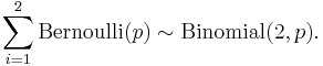
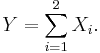
$\sum_{i=1}^2 \mathrm{Bernoulli}(p) \sim \mathrm{Binomial}(2,p).$

To show this let

$X_i \sim \mathrm{Bernoulli}(p), \quad 0<p<1, \quad 1 \le i \le 2$

and define

$Y=\sum_{i=1}^2 X_i.$

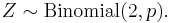
Also, let Z denote a generic binomial random variable:

$Z \sim \mathrm{Binomial}(2,p) \,\! .$

Using probability mass functions

As $X_1 \text{ and } X_2$ are independent,

$\begin{align}\mathbb{P}[Y=n]&=\mathbb{P}\left[\sum_{i=1}^2 X_i=n\right] \\ &=\sum_{m\in\mathbb{Z}} \mathbb{P}[X_1=m]\times\mathbb{P}[X_2=n-m] \\ &=\sum_{m\in\mathbb{Z}}\left[\binom{1}{m}p^m\left(1-p\right)^{1-m}\right]\left[\binom{1}{n-m}p^{n-m}\left(1-p\right)^{1-n%2Bm}\right]\\ &=p^n\left(1-p\right)^{2-n}\sum_{m\in\mathbb{Z}}\binom{1}{m}\binom{1}{n-m} \\ &=p^n\left(1-p\right)^{2-n}\left[\binom{1}{n}\binom{1}{0}%2B\binom{1}{n-1}\binom{1}{1}\right]\\ &=\binom{2}{n}p^n\left(1-p\right)^{2-n}=\mathbb{P}[Z=n] \end{align}$

Here, use was made of the fact that $\tbinom{n}{k}=0$ for k>n in the last but three equality, and of Pascal's rule in the second last equality.

Using characteristic functions

The moment generating function of each $X_k$ and of $Z$ is

$\varphi_{X_k}(t)=1-p%2Bpe^{it} \qquad \varphi_Z(t)=\left(1-p%2Bpe^{it}\right)^2$

where t is within some neighborhood of zero.

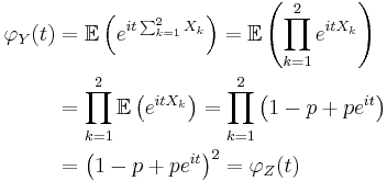
$\begin{align}\varphi_Y(t)&=\mathbb{E}\left(e^{it\sum_{k=1}^2 X_k}\right)=\mathbb{E}\left(\prod_{k=1}^2 e^{itX_k}\right)\\ &=\prod_{k=1}^2 \mathbb{E}\left(e^{itX_k}\right)=\prod_{k=1}^2 \left(1-p%2Bpe^{it}\right)\\ &=\left(1-p%2Bpe^{it}\right)^2=\varphi_Z(t)\end{align}$

The expectation of the product is the product of the expectations since each $X_k$ is independent. Since $Y$ and $Z$ have the same characteristic function, they must have the same distribution.

References

Hogg, Robert V.; McKean, Joseph W.; Craig, Allen T. (2004). Introduction to mathematical statistics (6th ed.). Upper Saddle River, New Jersey: Prentice Hall. pp. 692. ISBN 9780130085078. MR 467974. http://www.pearsonhighered.com/educator/product/Introduction-to-Mathematical-Statistics/9780130085078.page.